Turning to the sloping nature of elevation data related to postglacial rebound, we are confronted by a significant problem in that past research shows that rebound was characterized by uplift which is generally planar but perhaps locally was curvi-planar, that the planar inclination or slope apparently varies from place to place, and that the orientation of isobases likewise appears to vary spatially across the region. Further, these differences are matters of opinion which remain debatable and as yet unresolved. Thus, the state of knowledge about rebound is by no means settled.
Obviously, to apply the Bath Tub Model it is necessary to adjust the elevations of ice margin features to take into account the slope and isobase orientation aspects of isostatic rebound. Reported isostatic gradients in the region range from about 3 – 6 feet per mile(0.57 – 1.1 m/km). For example:
- Chapman(1937; 1939) shows strandlines on two north-south profiles, one for New York features and the other for Vermont features, in the Champlain Basin for multiple levels. These profiles indicate that the strandlines are basically parallel for Coveville, Fort Ann and the Champlain Sea at the marine limit, for example, with the gradient of the Champlain Sea at the marine limit with a gradient of about 4.3 feet per mile(0.8 m/km), flattening slightly at the Canadian border. Chapman also shows isobases which are oriented NE/SW. If the inclination of the sloping strandlines is measured perpendicular to his isobases the strandline inclination would be steeper, about 5.22 feet per mile(0.99 m/km). Chapman showed these strandlines sloping southward. Using the Quebec border Chapman(1937; 1939) shows strandlines on two north-south profiles, one for New York features and the other for Vermont features, in the Champlain Basin for multiple levels. These profiles indicate that the strandlines are basically parallel for Coveville, Fort Ann and the Champlain Sea at the marine limit, for example, with the gradient of the Champlain Sea at the marine limit with a gradient of about 4.3 feet per mile(0.8 m/km), flattening slightly at the Canadian border. Chapman also shows isobases which are oriented NE/SW. If the inclination of the sloping strandlines is measured perpendicular to his isobases the strandline inclination would be steeper, about 5.22 feet per mile(0.99 m/km). Chapman showed these strandlines sloping southward. Using the Quebec border as the reference point:
-
- Coveville 785 feet(239 m)
- Fort Ann 650 feet(198 m)
- Champlain Sea marine limit 490 feet(149 m)
- Port Kent 350 feet(107 m)
- Burlington 250 feet(76 m)
- Plattsburg 175 feet(53 m)
These elevations serve as references which can be related to ice margin levels.
2. Wagner(1972) presented a strandline profile giving similar elevations to those of Chapman. For example, his Fort Ann Lake Vermont strandline plot shows a range of elevations. In the Lamoille Basin his profile indicates Fort Ann elevations range from about 540 -600 feet(165 – 183 m), or an adjusted level at the Quebec border of 620 -680 feet(189 – 207 m). Wagner’s strandlines show a north-south isostatic gradient of about 5.1 feet per mile. He does not discuss isobase orientation but assumes the isobases are oriented east-west. 1Wagner’s Figure 3 shows multiple strandline data points with considerable scatter. As reported, most of these data points are from deltas with USGS topographic maps used for elevation control. As stated by Wagner, this strandline features entail elevation ranges, which introduces uncertainty in regard to the precision of strandlines. However, the Champlain Sea limit, which also includes the upper limit of mollusk shells, is relatively well defined. Usage of a gradient of 5 feet per mile for comparison of Wagner’s Champlain Sea delta point #72 near Enosburg Falls is marked are at an elevation of 440-460 feet, which when adjusted by a factor of 5 feet per mile gives an elevation of 495-515 feet. This compares with Wagner’s data point S2 near Weybridge at an elevation of about 175 feet, giving an adjusted elevation of 490 feet. If Wagner’s(1972) Champlain Sea strandline is correct, this gives a strong argument and support for using 5 feet per mile as the isostatic gradient for north south adjustments.
3. Calkin(1960s?,ibid, 15), who worked in the Middlebury area for S & M, reports the gradient as 4-6 feet per mile. This may be taken from Chapman.
4. De Simone and La Fleur(1985) 2 https://ottohmuller.com/nysga2ge/Files/1985/NYSGA%201985%20A10%20-%20Glacial%20Geology%20And%20History%20Of%20The%20Northern%20Hudson%20Basin,%20New%20York%20And%20Vermont.pdf for the southern Champlain Basin report concave upward curved strandlines, and gradients generally on the order of 2.4 – 2.7 feet per mile(0.45 m/km), but in more northerly areas show gradients of about 1.7 feet per mile(0.32 m/km) for Quaker Springs, 1.6 feet per mile(0.3 m/km) for Coveville, and 1.05 feet per mile(0.2 m/km) for Fort Ann, all with concave upward curvature.
5.Rayburn, De Simone, and Frappier(2018) show linear strandlines with a range of levels for Fort Ann due to changing outlet conditions.
6. Parent et Occhietti(1988, Figure 10) show the Fort Ann and Champlain Sea level at the International Border at elevations basically in agreement with Wagner’s levels for both of these strandlines, with a gradient of about 0.9 m/km = 4.75 feet per mile. These authors depict curved, arcuate isobases ranging from almost east-west in the Champlain Basin, to about N10E in the northeastern Vermont to about N45E in the Sherbrooke area.
7. Lewis, 2021, 3Lewis, C.F., 2021, Reconstruction of isostatically adjusted paleo-strandlines along the southern margin of the Laurentide Ice Sheet in the Great Lakes, Lake Agassiz, and Champlain Sea basins, from Figure 3 in: https://www.researchgate.net/figure/Map-showing-the-complex-of-North-American-ice-sheets-during-its-early-deglaciation-when_fig1_223056174. reports profiles indicating a regional isostatic gradient of 4.75 feet per mile( 0.9 m/km)( with nearly east west isobases for the Champlain Sea strandlines.
8.Franzi(2024 personal communication) finds a gradient of about 0.92 m/km = 4.9 feet per mile, with east west isobases in northeastern New York.
9. Wright(2024, personal communication) apparently utilized lower gradients than Wagner. However, the local elevation of the outlet for his Lake Winooski at 914 feet(279 m) as compared to the local elevation of Lake Winooski at a verified Wright location along the Worcester Range at 1080 feet(329 m), which is 29 miles(46 km) north of the outlet, gives a gradient along a north-south transect of 5.72 feet per mile(1 m/km). Wright regards the isobases in the interior upland area of Vermont as indicating a slight southeasterly slope.
The different estimates for isostatic gradients and isobase orientations are difficult to reconcile. Wagner’s(1972) strandline for the Champlain Sea maximum gives perhaps the best available data base, in terms of numbers of data points, and has the added benefit that the Champlain Sea marine limit is also marked by mollusk fossils. In this present VCGI report, the 5 foot per mile(0.95 m/km) gradient along a north-south transect is used as an isostatic correction factor, but the interpretations given by Chapman and Wright et al for identifying Lakes Winooski and Mansfield, and for correlating certain deltaic deposits with the Lake Coveville level are likewise relied upon.
Further, this report assumes and utilizes east-west isobases with isostatic corrections based on north-south transects. The difference between the NS transect versus, a slight NE-SW isobase orientation, as reported by others, results in only slight elevation discrepancies. Clearly, the matter of isostatic rebound deserves further study.
Whereas the entire matter of imprecision and uncertainty resulting from isostatic rebound, as just described, deserves further attention, in the final analysis, to put the issue into perspective, it needs to be recognized that the usage of the Bath Tub Model is not a highly precise exercise. It does not entail, nor does it require, precise elevations. As previously stated, all ice margin levels are reported as elevation ranges, which reflects the variability and uncertainty of the data used for establishing ice margin levels as ranges rather than precise, specific single elevations. For example, if in fact, the isostatic tilt is not 5 feet per mile(0.95 m/km) but closer to 4 feet per mile(0.76 m/km), the maximum “error” factor would be about 150 feet(46 m), given that the distance from the Canadian border to the Massachusetts border is about 150 miles(241 km). But the elevations of all ice margin features would be adjusted accordingly, likely leading to a similar correlation and ice margin chronology, regardless of the isostatic slope difference.
For example, the following is a screen shot of the VCGI map showing the T6 ice margin at a stagnant ice deposit west of Brandon:
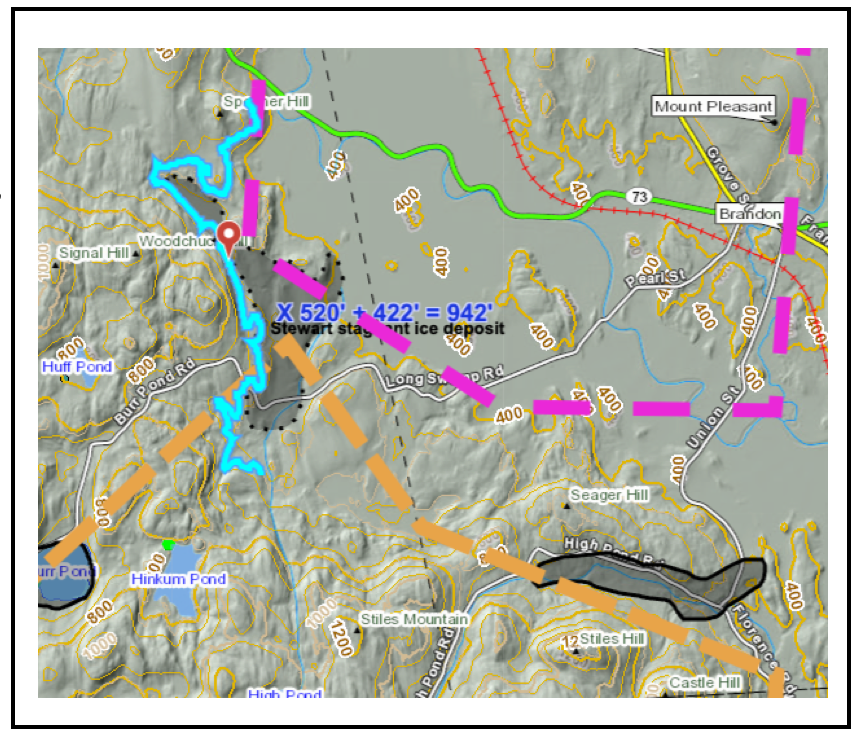
The elevation of this deposit is identified as being at 520 feet(159 m), which is shown by the highlighted contour on the screen shot. Using an isostatic correction factor of 5 feet per mile(0.95 m/km), the adjusted or corrected elevation is raised by 422 feet(129 m) based on the distance to the Canadian border of 84 miles(135 km), giving an adjusted elevation for the deposit of 942 feet(287 m), with the Canadian Border as the standard reference point. The elevation range used for the T6 ice margin is 800-900 feet(244-274 m). Whereas the adjusted elevation is 42 feet(13 m) higher than the T6 level range, the deposit was still correlated with the T6 margin, because this elevation is relatively close to the T6 level and fits with other features in the area at the T6 level. The point is that owing to imprecision and uncertainty the Bath Tub Model is not an exact science but is instead an approximation involving considerable subjective judgement.
If in the case of the Brandon feature the correction factor used instead was 4 feet per mile(0.76 m/km) the 520 foot(159 m) elevation would be raised by 338 feet(103 m) instead of 422 feet(129 m), giving an adjusted elevation of 858 feet(262 m) at the Border. Again, this elevation is still within the range of the T6 margin which is 800-900 feet(244 – 274 m). And again, all elevations would be adjusted.
Whereas the Bath Tub Model as used here is believed to be a valid basis for correlation and establishment of deglacial history, the merits of using the Bath Tub Model and isostatic rebound complications deserves further study.
Footnotes: